Hey guys, bring a pencil and a whiteboard next door. I want to show you something cool.

[Wave them over to the lab. At the front table, there are two tracks set up to make one long track (half of which is a ramp). Two carts and some extra masses (blocks) are at the ready.]

Are you ready?

Collision!

[The tracks are set up before us. I secretly and discretely check that the magnets in the carts are aligned so that they will attract (what a let down if they don’t stick together when you want them to!), leave one as the target on the flat track, and bring one up to the ramp to release. I put it in a specific spot, hold my finger in front of it, then move the finger.

An exciting collision!

And then, I try that again, but this time I put some extra mass in the incident cart. Another collision! But something’s different this time. Then again, a third time, but with the extra mass moved to the target cart instead.]

Hey, isn’t that sort of strange? The result is really different even though the total amount of mass is the same as last time.

So guys, what about this situation is new and what is basically something we’ve seen a lot of before? [The collision is new… we’ve seen carts going down ramps before. Plenty of times.] Okay, so what we really want to do, then, is find a way to understand, represent, describe… the collision.

Grab a whiteboard and a group; go model this for a few minutes

Let’s think about the very first collision that I showed you, where the carts have no extra masses in them. Let’s break up into a few groups with our whiteboards and model the situation. I’ll give you 8 to 10 minutes to draw some diagrams and represent what happened.

[After a packet chock full of goal-less problems in the last unit (unbalanced forces), they are ready to tackle that kind of prompt on their own. I basically left them alone and milled around checking out what conversations were happening. The focus when a lot of different places, but lots of FBDs, lots of velocity-vs-time graphs, and lots of talk about both going down a ramp and things hitting each other. Some talk about Newton’s 3rd Law. Etc. I’m not looking for anything in particular. I just want them to spend a few minutes dealing with the new situation on their own terms before we decide what to do next. I hope this makes them feel even more ownership over the experiment rather than feeling a bit led to it.]

Leave your whiteboards, but bring back your markers

[Collect back the markers so they don’t get lost around the lab. We’re not going to present or talk about our whiteboards, but this doesn’t bother anyone. They were doing some scratch goal-less thinking and are now ready to think about a goal.]

Okay, so we want to investigate the collision, right? That’s the thing we want to be able to represent better. So what can we measure that would help us better describe this situation?

[They pretty quickly zoom in on the masses and the velocities (before and after the collision).] So now we’ve got four quantities that we can measure and try to relate.

Mass of cart A — We can measure this easily in block because the carts have a mass of one block. We can get a lot of different data points by also using the half-block mass in combination with the other blocks.

Mass of cart B — Same as above.

Initial velocity (right before the collision) — We can measure this using the motion sensor at the end of the ramp. As long as we keep releasing it from the same height, we can just do a trial with no target cart and get the graph off of Data Studio. There is a button that gives you some data like max, min, and mean of the data you highlight.

Final velocity (right after the collision) — We can measure it using the motion sensor and the velocity graph from Data Studio (see above).

So of these four quantities, which can we easily change and choose values for? [The masses. With (possibly) a little prompting, they’ll realize they can just change the release spot to change the initial velocity.] So we can pretty easily choose everything except the final velocity. Does depend on the other three quantities? [Yeah.] So it sounds like we’ve got 3 experiments to do.

Then what are our objectives? To find a relationship between… [To find a relationship between… mass of cart A and final velocity… mass of cart B and final velocity… and initial velocity and final velocity.]

A purposely missing piece

We should probably think about this… couldn’t we also change the initial velocity of cart B? We’re choosing to always keep it zero. So when we put all of our results together, we’ll have to think about how we simplified things by purposely ignoring that aspect. We can already tell that combining these results is going to be a bit more complicated than piecing together .

[Of course, we’re also ignoring the possibility of the two carts having different final velocities, but that isn’t so obvious to the kids. Yet.]

Okay, let’s go take some data and make some graphs

Let’s do one experiment at each lab table. So the first table can change the mass of cart A, the second table can change the mass of cart B, and the third table can change the initial velocities. We’ll make some graphs and come together for a board meeting.

Be sure to measure each data point 3 times to check for consistency and get a range that you can put into LinReg. [One group was concerned that they didn’t have a range for the mass. I told them that since they made the measurement, they were the ones who had to report the range. They needed to find a way to do that. They ended up measuring the masses of the carts and blocks using an electronic balance and tried to figure out how much range there was on a measurement of “1 block”. So cool!]

When you’re done, head back to the classroom and make up a whiteboard with a sketch of your graph.

Board meeting: Time to really analyze the graphs and to get messy

Now. One group finds their experiment to go just as expected. The get a linear relationship. No problems. The other two groups find their results to be more frustrating.

Changing the mass of the cart on the ramp

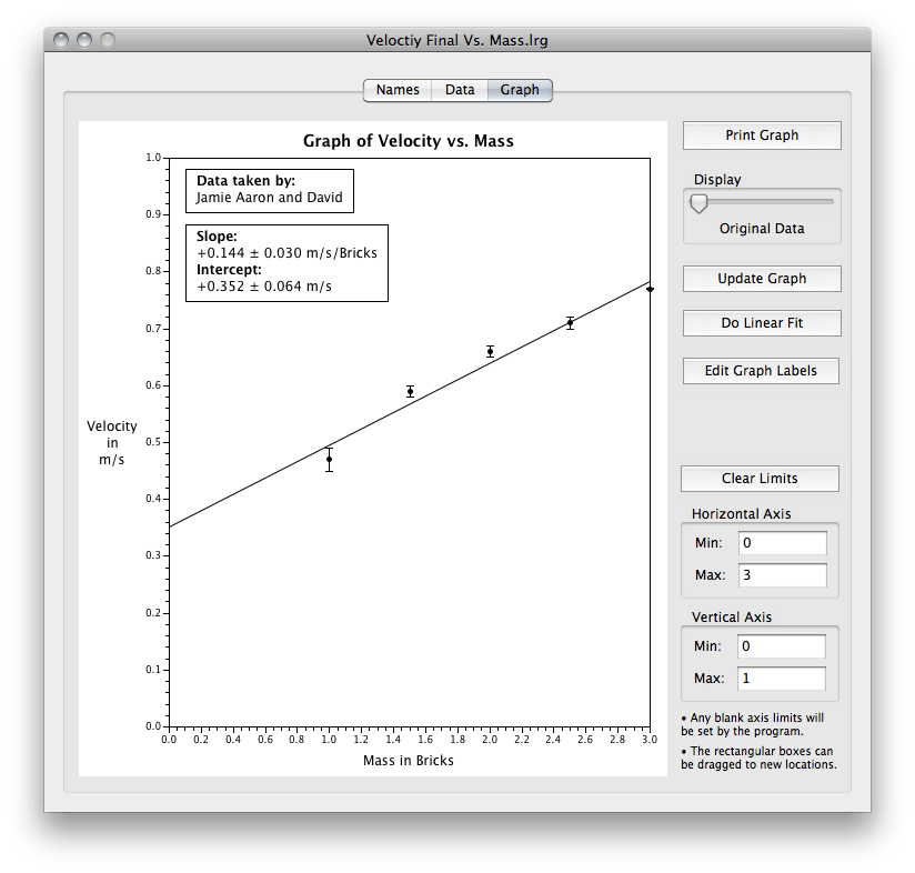
After navigating through the question of whether the initial velocity changes when the mass of the car on the ramp changes (Will we have to find a new release location each time we change the mass? Huh? It has the same speed no matter what mass we put on there? This is kind of weird…), the group gets into the groove and collects some nice data. They start to plot it and…

Meh. It’s sort of linear, maybe, with a cruddy data point in the mix. Or maybe two cruddy data points. Or something. But it doesn’t look much like any shape that we know. And, hey. Shouldn’t it go through 0,0? If there was no mass on the cart, would there be any kind of final velocity anyway?

Eventually, we come around to a question… is there a limit to the value of the final velocity? Or will the final velocity just keep getting faster and faster as we add more mass to the cart on the ramp?

Oh! There MUST be a limit! Because the carts are never going to end up going faster than the cart was originally going. The limit is the initial velocity. So this graph is shaped pretty strangely. It’s definitely a curve. It’s got an asymptote. It has to go through 0,0. This is not one of the function families or shapes of graphs that we know. It makes sense for the experiment, but it’s not handing us an easy relationship.

Changing the mass of the target cart

The first graph that they make looks strikingly familiar. It looks like the acceleration vs mass graph from the UBFPM experiment.

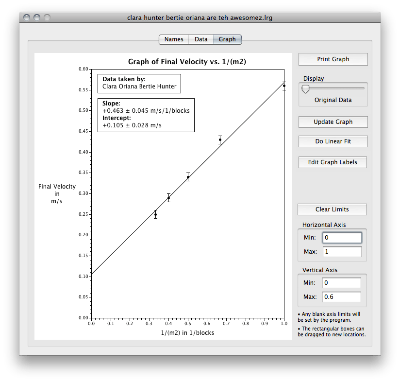
The students know just what to do to linear the graph. They plot the final velocity against the inverse of the mass. But what happens is…

…that they find this graph is also a bit frustrating. It looks really nicely linear for most of it, but there’s that nagging data point at the end. They retry that data point again and again, verifying their original data. They keep getting the same results. It’s just not linear.

Now that we’ve come together for our board meeting, though, they’ve seen what happened for the other mass-changing group, and they come to the same realization about the limit. The final velocity cannot be larger than the initial velocity in this case either. And this graph, also, should go through 0,0. If the mass waiting at the bottom of the ramp were very (infinitely?) large, the expected final velocity would be quite small indeed.

So this graph is also a curve, also goes through 0,0, also has an asymptote. It is also a shape that we just don’t quite know how to express with a function.

Changing the initial velocity of the ramp cart

Now this graph… this is a fine looking graph! It looks super linear, just as we always like to see. No need to do any calculations on the data to linearize the graph. Beautiful.

After analyzing the first two results, we wonder: is there a limit on this graph? Well, we suppose that strange things would happen if that initial cart starting getting near the speed of light, but within our ordinary cart experiences, a linear fit works well.

They tell me that the slope was “about one half” and I say that I find that pretty interesting. “Well I find that REALLY interesting, Ms. O’Shea,” retorts one of the kids from the group. Oh yes? Why? Well, there was one cart moving, then there were two carts moving with half the speed.

Whoa. Cool! Wait… does a pattern like that happen with other masses? So, for example, if you were changing the mass of the target, and now it had 2 blocks worth of mass, is the final speed about a third of the initial speed? Hey… yes! We went through a few of those, just looking at our raw data. We were starting to get a gut feeling for things, but it wasn’t neat and easy, and there was no elegant equation popping out that explained our graphs.

And then, we also remembered that we left out that piece of information from the beginning. We never considered what would happen if the initial velocity of cart B were changing, too. Man. It feels like we’re getting close, but we need some more data.

A murky pattern emerges

We need more data, and we definitely need some that includes initial velocities for both carts. We go back next door and set up a new track situation. We put a motion sensor at each end of the one track, and I do a bunch of experiments with the two carts. This time all bets are off on the initial and final states, so we try a lot of different things.

Some of the scenarios we tried:

• both carts moving in the same direction, colliding and sticking together
• “explosion” by using the plunger on one cart when both carts start at rest
• “explosion” when the carts are initially moving while stuck together
• variations on collisions where the magnets in the carts repel instead of attract, especially everyone’s favorite collision, the repelling magnet collision with equal mass carts

The kids brought in their whiteboards and markers, jotted down the data, and set to work looking for a pattern. We realized now that we had 6 variables (, , , , , and ), and we needed to find a way to relate all of them to each other. The groups responded differently. There was a great deal of concentration, a flurry of activity, some blank stares, and lots of drawing diagrams and trying things out. I try to stay out of the way.

 
 
 

Excitement starts to build as different groups start coming up with patterns. Not every group found a pattern, and most groups found different versions of the same idea.

One group looks at first at our original situation and comes up with and starts trying to do the same thing for a more general situation.

Another group calculates for each possible part and realizes that works for every case that we tried.

Still another group realizes that the masses are inversely related to the changes in velocities, and end up following out this reasoning (next to their ideas (left) is a top-down idea (right) that we started following at the very end of class that day):

Hey… …? Now that is starting to look like an elegant equation. And we are starting to look like quite the pattern hunters.

As we walked back into the classroom, the money student quote was, “I feel like that guy from A Beautiful Mind. Except without seeing imaginary people.” Does it get better than that??

Wait, did we just find Newton’s Third Law again?

So. We found out that the carts will have equal but opposite effects on each other.

Wait just one second there, mister. That sounds awfully familiar. In fact, as soon as we start talking about it, the cry went out in both sections, “Did we just do all of that work to find Newton’s 3rd Law?!”

Well, yes. And if we follow Newton’s 2nd Law (N2L) through (as we started on that board above), and add in Newton’s 3rd Law (Fnet on each cart is just the normal force the carts exert on one another… touching someone longer than they touch you we leave as a fun activity for dorm (appropriate touching!)… so the must be the same for each)… we see our observed pattern fall right out.

When we were using N2L, we were always considering one object at a time. It was a particle model, and we represented objects as a dot. We’re about to have a big paradigm shift, though. We’re going to consider multiple objects together as one system, and unlike other times when we’ve done that, these objects aren’t going to stay stuck together, move in the same direction, or have the same speed. This momentum business isn’t going to be a particle model at all.

Enter the IF charts

If our new model isn’t a particle model, we’re not going to be able to use particle representations (like free body diagrams) to think about it. We’re going to need something that lets us think about all of the objects in our system and that shows multiple snapshots (a before and after) rather than a single snapshot like we’d been using before.

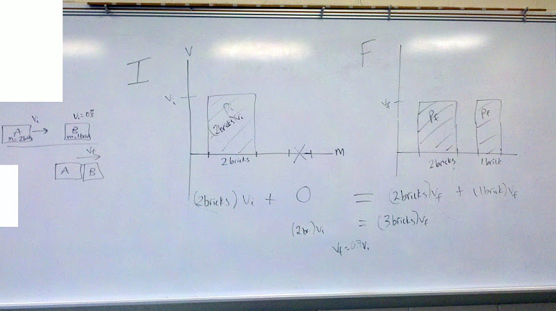
We need a new representation, and I propose a type of bar chart: IF charts. Here’s the example (the cut out parts of the photo were just other things written on the whiteboard that didn’t have to do with these charts) that we looked at during class.

IF charts (the IF is for Initial / Final… and they were named by a former student to distinguish them from the LOL bar charts that we use in energy (post on that coming later this semester) graph bars that have mass for their widths and velocities for their heights. That makes them cooler than the bar charts that you made back in 3rd grade because the areas have a physical meaning, too! The areas tell you the momentum of that object during that snapshot.

If there is no momentum transfered into or out of the system, then the charts are balanced, and the total initial area will be equal to the total final area. So it’s simple to write a straightforward equation for the conservation of momentum and to find anything you can’t find.

They even scale to 2-D problems (double IF charts… one for the x– and one for the y–components of the velocity and momentum).

These charts, though, are missing a piece telling you, if the charts are unbalanced, how unbalanced they are. That is, there is not an explicit component of the charts that shows momentum being transfered into or out of the system.

So, for my regular classes (who will be getting to this model after Christmas) and, assuming all goes well, for all of my classes next year, we’re going to try out IFF charts (if and only if charts?) which feature a third graph (a force vs time graph) that will indicate momentum being transfered into or out of the system.

At this point, I think IF charts merit their own individual post that can include a few examples, some of the common mistakes and confusions, and that can expand on the idea of double IF charts and IFF charts. So I’ll be making another post dedicated to IF charts, and I’ll link to that here when it’s ready. EDIT: And…. here’s the link! Momentum Bar Charts (IF Charts, IFF Charts).

Postscript

This year was my first try at doing the experiment this way, so I’ve only tested this on two classes so far (with two more to go in January). I used to do the impulse experiment of bouncing a cart off of a force sensor after we’d already broken down N2L into in the classroom (very close to the given MI experiment in the materials).

All of the above (up to the point where we introduced IF charts) took somewhere between 3 and 4 periods of 40 minutes each and was a great deal of fun (hopefully that was obvious!). Having finished the unit now, I think they have a better sense of when momentum isn’t conserved and how to figure out how “unbalanced” the IF charts will be (though I also changed which problems I put in the packet, so this experiment as well as the choice of problems… and, honestly, me just getting better at teaching this!… were definitely factors).